The expeditions in search of Sybaris, directed by Prof. F. Rainey (University Museum), have been conducted in collaboration with Dr. G. Foti (Superintendent of the Antiquities Department of Calabria), Eng. C.M. Lerici (Director of the Lerici Foundation of Rome), and Eng. and Mrs. E. Mueller (of Cassano Ionio). From these and from other organizations, the following persons participated actively in the 1964 program:
From the Superintendency: O. Miggiano and S. Pellegrion; From the Lerici Foundation: F. Brancaleoni, F. Serra, B. Pastore, U. Cesarini, and D. Achilli; From Cassano Ionio: G. Loisi, D. Falcone, and workmen; From Varian Associates, Palo Alto, California: S. Breiner; From the University Museum: F. Rainey, E. Myeller, D. Ridgway, and E. Ralph.
To these persons and organizations we should like to express our gratitude, and also to Mr. O. Bullitt of Philadelphia for his generous financial support.
For several years Dr. Rainey and various assistants have been looking for the ancient Greek city of Sybaris–not with eyes alone but with electronic, geophysical, and other accouterments. Now, at last, a new device has been developed, the Varian rubidium magnetometer, that may be capable of finding the city. But, even with the new assist from excited electrons, it is still not an easy job. Some of the reasons why Sybaris can not be found from an armchair with the help of the ancient references are these:
First of all, many scholars have studied the Classical sources (some have even received Ph.D.’s for their good work), and from these studies we now know about the lives, habits, habitations, and colonies of the Sybarites, but no one has been able to ascertain precisely where the city was.
Secondly, the plain of Sybaris–the region where Herodotus and others said the city should be–is very large, approximately eighty square kilometers and the archaic sixth century B.C. city is buried at great depths, five to six meters.
Thirdly, sites where the descendants and the predecessors of Sybarites may have lived have been found in the surrounding hills. With these included, the area of search becomes many times larger.
Fourthly, Sybaris was destroyed by the un-neighborly Crotoniates in 510 B.C. In that fateful year, according to Strabo, it was buried by diversion of one of the rivers, the Crati or the Coscile, but it may not have been buried completely or, if so, not deeply enough to prevent the Greeks who started building again in the fifth century from mixing up some of the evidence. Fortunately, in regard to making our task easier, these inhabitants of the fifth century B.C. gave their new city a new name–Thurii. To compensate for this facileness, however, the Thurians built their city at approximately the same elevation as that of Sybaris. Even though our instruments and their operators are now well trained, it is difficult for them to differentiate between the buried walls of Sybaris at depths of 4 1/4 to six meters and those of Thurii which might be immediately above or, at comparable depths, resting on their own underpinnings.
The Romans, naturally, followed along later and named their city Copia Thurii. Fortunately for our instruments, many of the Roman structures are massive and extend upward to within one to three meters of the surface. Therefore they are much easier to detect and may be distinguished from their more elusive Greek forerunners by the magnitudes of the magnetic anomalies.
Fifthly, the elusiveness of Sybaris is increased by the high water table. The sybaritic level of occupation is at least three meters under the fresh-water table, and well below the present sea level. This may have been caused by various disturbances, but most likely from tektonic movements which initiated tilting of the land, subsequent blocking of water bodies, consequent deposition of great quantities of fine blue-gray-green clay, and concordant land subsidence.
The soil and water conditions, in combination with the depths of the structures sought, dictate the types of instruments to be used. On the plain of Sybaris the water table is higher than all but the highest remaining Roman constructions. Therefore, electrical resistivity methods are ruled out. instruments based on wave propagation such as standard geophysical seismic detectors function well to find earth layer changes, as they are designed to do, but the long wave lengths associated with the low seismic frequencies bypass without “seeing” the comparatively small archaeological features above them. Sonic detectors, operating at frequencies higher than seismic, offer possibilities, but are not yet ready for field use. The important basic method of detection which remains and which is applicable for the deeply buried structures on the plain of Sybaris is that of magnetic contrast.
As a result of nuclear and other research conducted for entirely different purposes, there are detectors of magnetic intensity available that are rapid and easy to use. Proton magnetometers have now been employed for archaeological prospecting for several years and the Oxford Elsec instrument made by the Littlemore Scientific Engineering Co., oxford, England (see M.J. Aitken, Physics and Archaeology, Interscience Publishers, 1961) was designed specifically for this purpose. The Oxford units are capable of measuring changes of one gamma, which is a small unit in magnetic parlance (10 -5 oersteds), but on the plain of Sybaris, it is not quite small enough for the detection of the deeply buried archaic Greek structures where the magnetic contrast between walls and earth is comparatively small.
Eventually, the next step was to find or develop an instrument with greater sensitivity. But, as with many obvious things, there were complications such as natural diurnal magnetic variations of magnitudes comparable to the anomalies sought, shorter micro pulsations, variations due to uneven ground, etc. However, many of these disadvantages have become overcome or circumvented with the new Varian rubidium magnetometer. (See V-4938 data sheet, Instrument Special Products, Varian Associates, 611 Hansen Way, Palo Alto, California.)
The Varian rubidium magnetometer was designed primarily for measuring the earth’s magnetic field from planes, rockets, and satellites. Our joint tests (in Canada in May and in Italy in October) were among the first both to assess the applicability of an instrument with greater sensitivity for archaeological prospecting and to determine what arrangement of and what changes in components are needed for this adaptation.
The rubidium magnetometer is more sensitive than the proton magnetometer because of the fact that for a given magnetic change, the resultant change in frequency–the property that the instrument detects–is a hundred times greater. The two types of magnetometers detect this information in different ways, both of which, however, are based upon energetic movements within atoms. The proton magnetometer is so named because protons in the alcoholic detector bottle (after an initial “upset” with an artificial magnetic field supplied in a surrounding coil) gyrate at speeds that are proportional to the earth’s magnetic field. The rubidium sensor is appropriately filled with rubidium, which, when heated above room temperature, happens to be both a vapor and to have well-defined lower energy states. The changes in energy levels, due to magnetic changes, are, therefore, more readily detected. In use, the electrons are first disturbed by a so-called optical frequency. After this upset, the energy levels which are, in effect, the residences of the electrons, are readily “split” into sublevels and the amount of splitting is dependent upon the magnetic intensity beneath the rubidium sensor. The splitting is measured as a frequency which corresponds to the difference in energy between two particular sublevels. For the isotope Rb85 the resultant frequency change due to the separation between sublevels is one hundred times greater than the gyration frequency of the protons for a unit change in magnetic intensity.
Theoretically, the proton magnetometer is capable of detecting changes of one gamma, but, in practice, only a change of four gammas or more provides usable information. This could be reduced with dual detector arrangements and more elaborate circuitry, but with consequent loss of portability (i.e. my aching back!). In addition to the extra sensitivity available in the rubidium instrument, the fact that readings are taken continuously (and recorded) enables us to survey a given area about four times as fast.
It should now be easy to find the archaic Greek walls. In practice, however, in these initial tests, there were more pitfalls than progressions. The first test of the rubidium magnetometer was planned over the Long Wall, a known anomaly. The recorder and circuits were not yet battery-powered so that this was also the first test under load of a second-hand generator which I purchased in Rome. Our first problem was apparent immediately. The generator’s speed, voltage, and frequency were all variable, and variable additionally when the load (that is, the instrument) was attached. This latter variation created a bad problem because it necessitated the setting of the voltage too high at the start, so that when the instrument was attached, its load would cause it to drop to the proper operating value. This was unsafe, however, for the rubidium magnetometer because it permitted the application of an overvoltage before its circuits were warmed up and drawing their usual load of current. To do it the other way around was more hazardous with this particularly bad generator–that is, to attach the magnetometer and then raise the voltage–because the voltage control was not linear nor stable. When varied, it tended to jump suddenly from minimum to maximum voltage, a jolt certain to wreck the magnetometer.
One way around this was to preset the voltage, as suggested, and to attach additional loads which could then be removed as the magnetometer warmed up. This we did, but since this was our first day of field tests and we had not brought with us every possible spare part, our subsidiary loads of soldering irons were insufficient. Result: Bang! Fuse blown in magnetometer. Another try–fuse blown again! (which indicated that the problem was more serious than just a fuse). Our volt-ohmmeter, or “tester” ( a small handy gadget for trouble shooting) revealed that there was no impedance in the input circuit. Obviously, with out over-voltage we had burned out something–a component possibly as serious and specialized as the main power transformer.
The generator then ceased temporarily to be the black monster because, with it, we had power for a soldering iron and could disconnect wires–vital for trouble shooting. With great relief we soon found that the bad actor was a diode in the rectifier–not quite so irreplaceable in Italy. Still some question of whether we could find a similar diode, a small semiconductor that is quite a modern electronic component. We were lucky for, in the radio and TV supply shop in the small town of Trebisacce, there was one.
On the next day we were more cautious and attached electrical loads of light bulbs and more soldering irons before connecting the magnetometer. We included also a voltage regulator in the power line but, by some mischance, we managed to burn out the regulator before it proved its usefulness. With the voltage now under control, we resumed our initial tests over the Long Wall. It soon became apparent, however, that the frequency of the voltage that the miserable generator grudgingly produced was not right for the recorder. With a rapid instrument such as this, a requisite is a lively recorder, but, on the contrary, ours was “lentissimo.” It took us a while to find out how to adjust the speed of the generator, mostly because the control was broken. When this was realized, and after another half-day’s delay while a new part was made in Candido’s excellent machine shop, some adjustment of the frequency could be made which enabled the recorder to have some “life”–not optimum, but operable.
On the third day, therefore, with the new rubidium magnetometer, we detected our first anomaly–a large peak in the recorder graph which appeared as the movable sensor was carried perpendicularly over the Long Wall. (This was easy to find since this wall is sufficiently massive to have been located previously with the proton magnetometer.) This was encouraging, however, because, if the recorder paper had been wide enough, the anomaly might have appeared a hundred times larger than with the proton magnetometer. Since the paper was of limited width, the needle, of course, went off-scale until the gain (or amplification) of the instrument was reduced by about one twentieth of maximum.
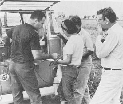
We were then ready for the first real test. Could the less massive, more deeply buried walls be located with the rubidium magnetometer? Two logical places to start the search were the “ends” of the Long Wall, that is, the regions where it was “lost” by the proton magnetometer. Before we had collected all of the pieces, parts, and apparatus that we had strewn around the field at our first test site however, rain descended. It does not rain in Calabria in October but this was an unusual year. In fact, it had already been raining off and on in September–an occurrence that never happens. Therefore, we felt the need to make ourselves and the equipment both more portable and more rainproof. We, therefore, arranged the main part of the instrument on the back shelf of our Volkswagen Microbus so that the operator could recline on the back seat inside and be protected from both wind and rain. More important, the most expensive part of the apparatus was protected and we did not lose the results which the recorder plotted as graphs in water-soluble ink. Remaining outside were the generator (noisy, odorous, and of less value), the two sensors, and the squawk box. This last consisted of a small but forceful amplifier and speaker which broadcast the resultant rubidium frequencies audibly for the benefit of the man who moved the sensor, who had necessarily to be at a distance from the rest of the apparatus which was not free of iron and other makers of magnetic anomalies. The sensor man could then hear the anomalies as he passed over them and, by hearing the changes in frequency as well as a steady signal from regions without anomalies, he could both be sure that he was carrying the sensor at the correct angle and keep his attention on the job by knowing when he had found anomalies. Unlike the proton magnetometer, the rubidium sensors are somewhat sensitive to orientation with respect to the magnetic north pole. There are certain solid angles in which they work and others in which they do not.
After more rain, during which Breiner adjusted the sensors, the vital rubidium-filled detectors, which had the bad habit of being either too hot or too cold, we were ready for serious work on the fifth day. The procedure was then as follows:
- Drive Microbus into edge of area to be surveyed.
- Unload generator and its special “loads,” lay out 400 feet of cable for the movable sensor, and unload sensors and squawk box.
- Put gasoline and oil in generator (like an old car, it consumed both).
- Start generator with “loads.”
- When warmed-up and stable, connect instrument and recorder. As voltage drops, remove loads as needed to reach proper operating voltage (some loads remain to help stabilize things).
- Wait 15 to 30 minutes for sensor heaters–necessary items to vaporize the rubidium–to warm up. (When all is in order one hears a distinctive frequency from squawk box.)
- Everything ready–rain begins.
- Wait 1 to 2 hours.
- Repeat steps 1 to 6.
- Ready again. Lunch time.
- One hour later–ready again.
- Generator runs out of gas–forgotten.
- Repeat steps 1 to 6.
By mid-afternoon a few trial lines were run in a cow pasture beyond the southeast “end” of the Long Wall. These were interrupted, at last, only by the passage of the cows who naturally selected the spot where we were to pass en masse on their way to the barn. We had selected this pasture because it was one of the fields that wasn’t too muddy to drive into. (Even so, after one particularly rainy morning, the Microbus had to be pushed out by six men.) The pasture, however, proved to be a fortuitously good hunting ground because we began to detect anomalies of both small and large magnitude. The next step was to make measurements on a grid, a series of parallel lines equal distances apart, so that the results could be plotted in a quantitative way.
Franco Brancaleoni kindly surveyed and staked out a large grid, 90 x 120 meters, for this purpose. With lines run three meters apart, we then ran measurements along 40 lines, each 90 meters long. As the sensor was moved over each line, a graph, representative of the 90 meters covered, appeared on the recorder. This large grid was completed in two days and only two Volkswagen “stations” were required–that is, one more after the initial location. Without breakdowns, rainstorms, etc., it could be completed in less than a day and, at least four times faster than with the proton magnetometer. Unfortunately, when the final plot of the results was made (as it happened, six weeks elapsed; but much less time will eventually be required for this) it was found that a shift had occurred within the instrument at some unknown time in the course of doing this large grid. Therefore, the grid could be plotted only with countour intervals of two gammas rather than one or less. In other words, some of the extra available sensitivity, one of the big advantages of the rubidium versus the proton magnetometer, had been lost.
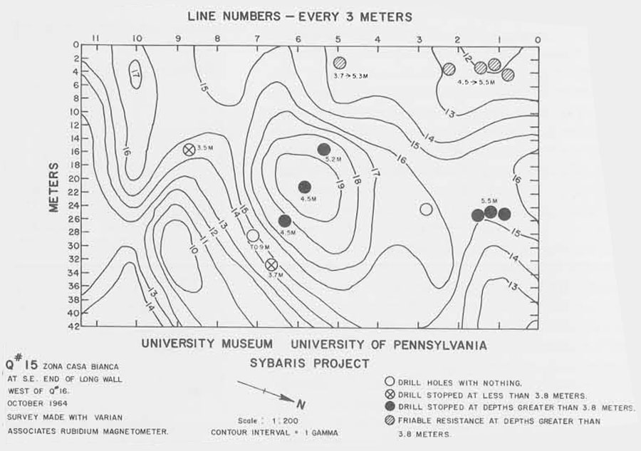
This fault did not occur, however, for Grid #15, a much smaller one. It is seen in the plot of this grid that anomalies (the circular patterns such as the one of 19 gammas maximum in the center of the figure) represented by changes as small as three gammas were detected. These more or less circular shapes have been found, in many cases, to be representative of buried structures. This deduction is confirmed for the central anomaly by the drill results. (The use of drills has been reported by D.F. Brown, Expedition, Vol. 5, No. 2, 1963.) It is not clear why a structure was found also in the north central part of the grid not coincident with the center of the anomaly nor with the magnetic contour gradients. One possible explanation is that this structure was found at a depth of 5.5 meters, whereas that in the center of the central anomaly was struck at 4.5 meters, that is, one meter closer to the surface. The fact that these regions have positive magnetism may indicate also that they are caused primarily by concentrations of roof tiles (magnetic materials). It is unfortunate that the central portion of the larger non-magnetic anomaly represented by a lowering of the magnetic intensity to ten gammas (southeast corner of the grid) was not tested by drilling. From previous experience with the proton magnetometer and also from the drill results at the base of the anomaly, one might guess that this non-magnetic disturbance represents a structure of stone buried less deeply.
One may wonder why we do not use drills along instead of bothering with such fastidious electronic apparatus. The answer is mainly that, if a drill misses a wall by one centimeter, it says: “No wall,” but the sensor of the rubidium magnetometer may miss the wall by three meters and still detect the anomaly caused by it. In other words, for the particular application on the plain of Sybaris, the rubidium magnetometer affords a means of plotting the buried structures in the form of a magnetic map of the region of interest without drilling or excavating every square meter of earth. To accomplish this for an area of nine square kilometers, a year of continuous work might be required but this, even so, is a small amount of time for mapping a city of the fame of Sybaris.
How do we know whether the anomalies are representative of Greek or Roman times? In most cases, those from Roman structures are very much larger because they are generally massive and closer to the surface. Here again, a few test drill holes made in strategic spots after the anomaly is located, will indicate the depth and, by the pottery nearby, the age of the level of the top of the wall. Since the difference in levels between Sybaris of the sixth and Thurii of the fifth century B.C. is not great, a few test excavations may be required.
When this survey has been made, and when we, therefore, know the extent and location of the zone of deep structures, it may then be possible to answer the question: WHERE IS SYBARIS?